PID Tuning for Chemical Process Control Loops
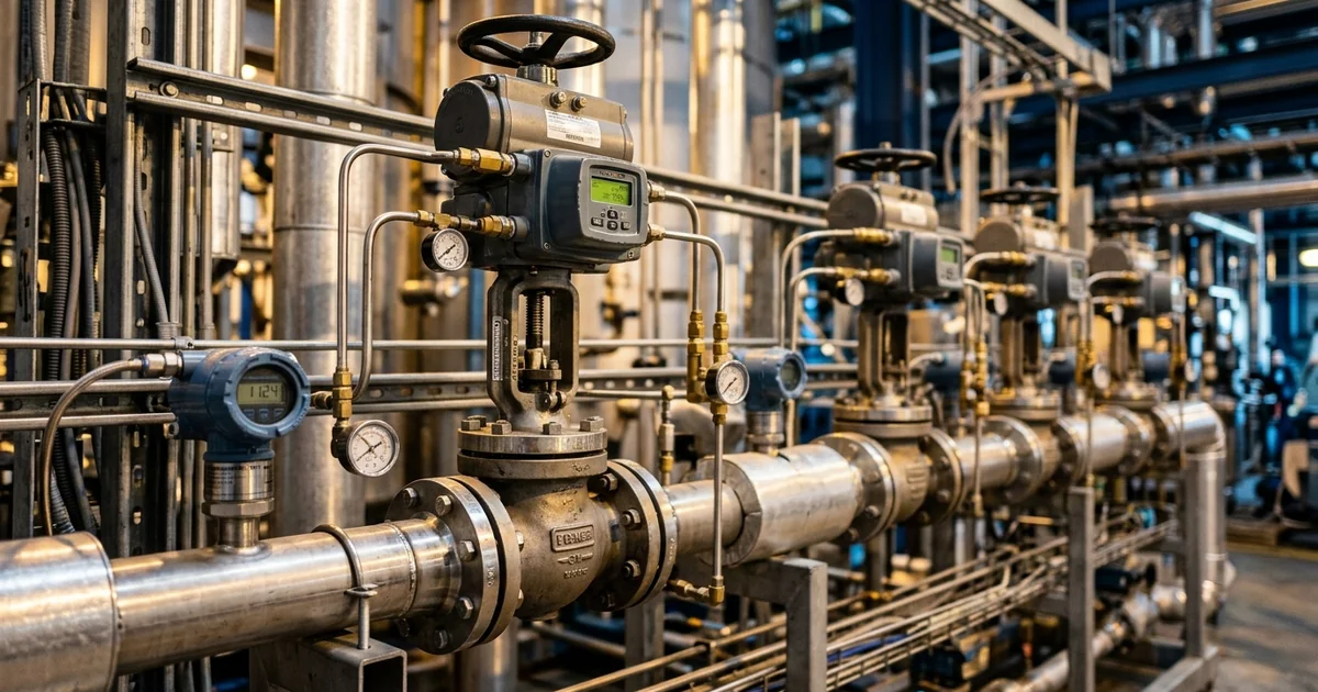
A reactor temperature loop that cycles gently around its setpoint looks harmless on the trend screen. On the plant it wears the control valve, stretches the heat-up phase and lets a dosing step push the batch past the temperature the product tolerates. Skogestad observes in his 2003 tuning paper that a visit to a process plant usually shows a large number of poorly tuned PID controllers. This guide to PID tuning process control shows how to read a loop's dynamics, compare the Ziegler–Nichols, Cohen–Coon, lambda and SIMC methods, and separate tuning faults from hardware faults. It draws on the published tuning literature and on the automation and control scoping work Global Formulation supports for plant owners.
PID Tuning Process Control Basics: What P, I and D Each Do
Every PID controller turns one number, the error between setpoint and measurement, into one output to the valve. Three settings decide how it does that, and each trades speed against stability in a way the plant feels directly. Knowing what each term does tells you which setting to touch when a loop misbehaves. The list below sets out the three terms and the plant consequence of getting each one wrong.
- Proportional — output moves in proportion to the present error, set by the controller gain (Kc) or its reciprocal, the proportional band. Too little gain leaves the loop sluggish, while too much makes it oscillate and keeps the valve in constant motion.
- Integral — output keeps changing until the error is zero, set by the integral time (TI). It removes steady offset, but a fast integral term causes slow overshoot cycles and, once the valve saturates, integral windup.
- Derivative — output responds to the rate of change of the measurement, set by the derivative time (TD). It speeds up slow, lag-dominant loops such as reactor temperature, but it amplifies measurement noise and makes a valve chatter on a noisy signal.
Before any of these settings can be chosen, the loop's own behaviour has to be measured, which is the subject of the next section.
Read the Process First: Gain, Time Constant and Dead Time
A tuning method is only as good as the model behind it. Most model-based tuning methods start from the same three numbers, which describe how the measurement responds when the controller output is stepped. Measuring them takes a short test and replaces guesswork with data. The same numbers also explain why settings from a bench reactor fail on a plant vessel.
The first-order-plus-dead-time (FOPDT) model underpins most PID tuning rules for self-regulating loops, and it uses three parameters, shown in the figure below. Process gain (K) is the steady change in measurement per unit change in controller output. A time constant (τ) measures how long the measurement takes to cover about 63% of its final change once it starts moving. Dead time (θ) is the delay between the output step and the first visible response.
A step test, often called a bump test, is the standard way to gather data for PID tuning. It has four parts:
- Hold the process steady — put the controller in manual so the response reflects the process and not the controller.
- Step the output — make one small change in controller output and leave it alone.
- Record the response — log the measurement until it settles at a new steady value.
- Read the three numbers — take gain from the final change, dead time from the delay, and time constant from the time to reach about 63% of the change.
A step test on a live reactor loop belongs inside the site's change and permit procedures, with the step size agreed with operations and process safety. The step must be small enough to keep the batch in its normal envelope and large enough to stand out from noise.
Dead time sets the ceiling on achievable performance, because the controller cannot see the effect of its own action until the delay has passed. Skogestad's robustness guidance sets the closed-loop time constant no lower than the dead time. A thermowell, a long sample line or an analyser cycle all add dead time that no setting can remove.
Scale changes all three numbers. A plant vessel has far less heat-transfer area per unit volume (A/V) than a bench reactor. Its thermal time constant therefore grows, and settings from the lab do not transfer. Our guide to scale-down models shows how to design bench work that predicts plant behaviour. The gain itself also shifts with valve characteristic, vessel level and batch temperature, so the step test must run at the operating point where the loop will actually work.
With the three numbers in hand, the loop type decides which terms the controller should use at all.
PID Settings by Loop Type: Flow, Level, Pressure, Temperature and pH
Loop type decides most of the tuning strategy before any test is run. A fast flow loop and a slow reactor temperature loop need opposite priorities, and applying one recipe to both is a common source of trouble. The table below summarises how dynamics and term use differ across five loop types found on a batch plant. Read it as a screening guide and confirm each loop with its own step test.
| Loop | Typical dynamics | Usual terms | Main tuning concern |
|---|---|---|---|
| Flow | Fast, self-regulating, noisy signal | PI, derivative normally left out | Valve resolution and measurement noise limit how high the gain can go |
| Gas pressure | Fast, driven by inflow and outflow valves | PI | Interaction with flow loops on the same header |
| Liquid level | Integrating, with no natural steady state | P or PI | Tight tuning passes upsets downstream, while averaging tuning uses the vessel as a buffer |
| Temperature | Slow and lag-dominant, with dead time from sensor and jacket | PID where a second lag exceeds the dead time, otherwise PI | Heating and cooling asymmetry, windup on ramps, and the need for cascade |
| pH and composition | Strongly nonlinear, with long dead time | PI with gain characterisation | Process gain changes sharply across the measurement range |
Level loops need separate treatment because they integrate the difference between inflow and outflow, so they have no natural steady state. Skogestad notes that lambda tuning does not apply to pure integrating processes, and that the SIMC rule extends the same approach to them. Averaging level control tuning uses the vessel as a buffer so that downstream units see a smoother flow, while tight tuning passes every upset straight through.
PID settings for reactor temperature control start from the dominant lag, and derivative action earns its place only where a second lag exceeds the dead time. On jacketed reactors, a cascade structure splits one slow temperature loop into a fast jacket loop and a slower reactor loop. The inner loop is tuned first and the outer loop second, as set out in our guide to cascade temperature control of jacketed reactors. Dosing-controlled semi-batch reactors link the feed loop to the temperature loop. Reactor configuration therefore becomes part of the tuning problem, as our guide to batch, semi-batch and continuous reactor selection explains.
Once the loop type is clear, the remaining choice is which tuning method to apply to the measured model.
PID Tuning Methods Compared: Ziegler–Nichols, Cohen–Coon, Lambda and SIMC
Five families of tuning rules cover most chemical plant practice, and they differ in what test they need and what they let the engineer choose. The useful comparison is not which gives the best response on paper, but which gives a defensible response on a loop with dead time, noise and a sticky valve. Skogestad's paper describes Ziegler–Nichols settings as aggressive and the IMC-based rules as robust. The table compares the methods on the points that matter on a plant.
| Method | Test needed | What you choose | Strength | Limitation on chemical loops |
|---|---|---|---|---|
| Ziegler–Nichols (1942) | Closed loop: raise the gain until the loop oscillates steadily, then read ultimate gain and period | Nothing, because the rules are fixed | Needs no process model, and gives a good disturbance response on integrating processes | The test drives the loop to its stability limit, the settings are aggressive, and dominant dead time degrades performance |
| Cohen–Coon (1953) | Open-loop step test (reaction curve) | Nothing, because the formulas are fixed | Built around a first-order process with dead time, and needs no oscillation | No parameter for trading speed against robustness |
| Lambda tuning | Open-loop step test | λ, the desired closed-loop time constant | The engineer sets loop speed directly | Undefined for pure integrating loops such as level |
| SIMC | Open-loop step test, with the half rule to reduce higher-order models | τc, the closed-loop time constant | Gives the lambda PI rule for first-order-plus-dead-time loops and extends to integrating loops | Needs a usable model, and the engineer must still choose τc |
| Relay autotuning (Åström–Hägglund, 1984) | Closed loop: a relay generates a sustained oscillation | The rule built into the tool | Automates the ultimate-gain test inside the controller | The result depends on the tool's rule and a clean test, so it still needs review |
Rules with a tuning parameter are easier to defend, and four comparisons come up most often on plants. Ziegler–Nichols vs Cohen–Coon is mainly a choice between a closed-loop oscillation test and an open-loop step test. Open-loop vs closed-loop PID tuning is a question of risk. A step test leaves the controller in manual, while an oscillation test pushes the loop towards its stability limit. Ziegler–Nichols vs lambda tuning turns on the tuning parameter, because lambda and SIMC give the engineer one number to choose, as Skogestad's note on the history of these rules explains. Lambda tuning vs SIMC differs only for integrating loops, which lambda tuning cannot handle. The lambda rule traces to Dahlin's 1968 direct-synthesis idea. Setting λ equal to the dominant open-loop time constant, a conservative start, appears in the 1986 IMC-PID paper of Rivera, Morari and Skogestad. Many built-in autotuners automate the relay test, yet the engineer still owns the choice of closed-loop speed.
For a first-order-plus-dead-time loop, the published SIMC PID tuning rules reduce to a short proportional-integral pair. Controller gain is Kc = (1/K) × τ / (τc + θ). Integral time is TI = min[τ, 4(τc + θ)], where τc is the chosen closed-loop time constant. Skogestad's first choice is τc equal to θ, which gives a reasonably fast response with good robustness margins, and a larger τc detunes the loop.
Treat the formula as a method, not as a setting. Its inputs must come from the loop's own step test, and the result is checked in the plant before it is accepted. The PI vs PID control decision follows the process. A derivative term is added only where a second lag exceeds the dead time, because that is where derivative action pays for its noise sensitivity.
Integral Windup, Derivative Kick and Anti-Windup Settings
Correct PID tuning numbers can still produce bad behaviour when the controller's implementation details are wrong. Two faults are common on batch plants: integral windup during long ramps and derivative spikes after setpoint changes. Both come from how the algorithm treats a saturated valve or a stepped setpoint, not from the gain settings. Fixing them takes a configuration check rather than a retune.
- Integral windup — when the output saturates, for example the heating valve at full open during a ramp, the error persists and the integral term keeps accumulating. The stored value holds the valve at its limit after the measurement crosses the setpoint, so the batch overshoots until the integral unwinds.
- Anti-windup — the standard methods are conditional integration, limiting the integral term, and back-calculation. Modern DCS and PLC platforms make windup prevention a configuration matter, so the fix is a setting rather than new hardware.
- Derivative kick — a stepped setpoint produces a spike in the derivative term. Most commercial controllers therefore base derivative action on the measurement rather than the error, and a low-pass filter on the derivative term limits noise amplification.
- Setpoint weighting — proportional action on a setpoint step jolts the output. Weighting the setpoint in the proportional term softens that response, and batch recipes often ramp setpoints instead of stepping them.
A tuning that passes a small step test at mid-range can still wind up on the first full heat-up. Test the saturated case as well as the linear one, and the overshoot is found during commissioning rather than in a production batch.
Troubleshooting a Control Loop That Oscillates, Hunts or Responds Slowly
Most calls about a control loop oscillating or responding slowly reduce to a few recognisable patterns, and only some are cured by retuning. A University of Alberta study lists improper tuning, multi-loop interactions, sensor faults, external oscillatory disturbances and control valve problems as the sources of oscillation. It reports that valve stiction appears to be the main cause in 20–30% of oscillating loops, citing earlier surveys. Sorting the cause first prevents hours of retuning a loop whose real fault is mechanical.
| Symptom | Probable cause | First check |
|---|---|---|
| Regular cycling while the valve moves smoothly | Gain too high, integral too fast, or dead time longer than in the tuning test | Repeat the step test and compare it with the model behind the current settings |
| Limit cycle that survives retuning | Valve stiction or deadband, where the stem does not move although the controller output keeps changing | Run a small-step valve test as defined in ISA-75.25.01, then inspect packing and positioner |
| Several loops cycling at the same period | Loop interaction or a shared external disturbance | Find the common source, such as a shared header, before retuning any single loop |
| Overshoot after a long ramp or startup | Integral windup while the output was saturated | Check the anti-windup and output-limit configuration |
| Valve chatter and a noisy controller output | Derivative action on a noisy or unfiltered measurement | Base derivative on the measurement, add a filter, or remove derivative action |
| Sluggish control loop response, with slow creep back to setpoint | Gain too low or integral too slow for a lag-dominant process | Compare with the step-test model and shorten the integral time within the robustness limit |
| Output pinned at 100% with the measurement short of setpoint | Insufficient capacity, not a tuning fault | Check heat-transfer and cooling duty against reaction calorimetry data |
| Stable at one load but cycling at another | Process gain changed with operating point or valve characteristic | Test at both ends of the range, then add gain scheduling or valve characterisation |
The saturated-output case deserves emphasis because no controller setting can deliver heat-transfer capacity the equipment does not have. When the output sits at its limit with the measurement short of setpoint, the loop is reporting a capacity limit and the investigation moves to the duty. That is where thermal data from calorimetry belongs, and retuning only hides the shortfall.
A PID Tuning Workflow for Chemical Plant Loops
PID loop tuning goes faster and lasts longer when it follows a fixed order. The order matters because hardware faults and wrong algorithm settings both masquerade as tuning problems. Each step below removes one class of fault before the next is attempted. The sequence ends in a record the next engineer can audit.
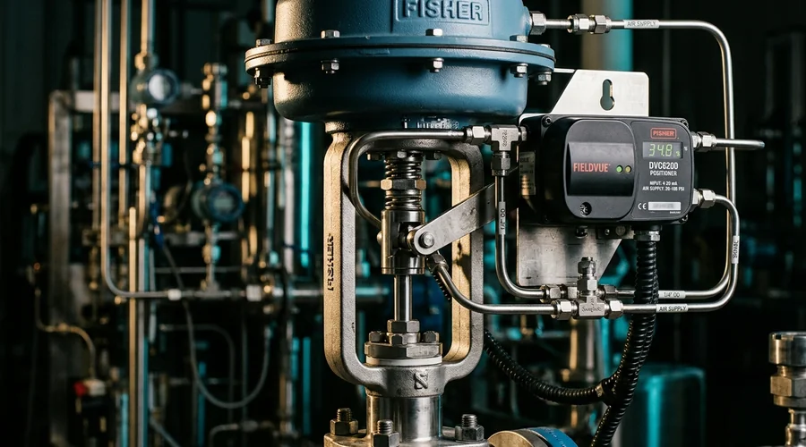
- Check the hardware first — confirm valve response, measurement lag and sensor location before touching a setting, using a small-step valve test where stiction is suspected.
- Define the objective — decide whether the loop must track setpoint changes tightly, reject disturbances, or absorb them, as an averaging level loop does.
- Measure the process — obtain gain, time constant and dead time from a step test at the operating point, inside the site's change procedure.
- Choose a method with a tuning parameter — lambda or SIMC, with the closed-loop time constant no shorter than the dead time.
- Confirm the algorithm form — match standard, parallel or series form, and the units of gain and integral action, to the controller in use.
- Enable windup and kick protection — set anti-windup, measurement-based derivative and a derivative filter before the loop goes to automatic.
- Verify and record — confirm the response to a setpoint change and a load change across the operating range, then file the settings and the step-test model under change control.
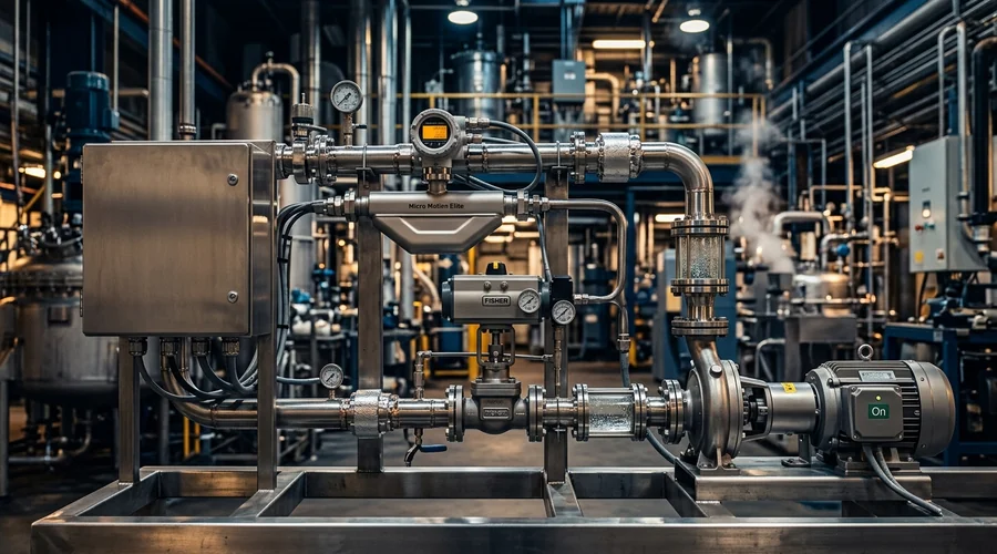
Where loops keep cycling after this sequence, look at structure rather than settings: a missing cascade, an undersized valve or a measurement too slow for the duty. Those are the questions an automation and control scoping study answers. Our process engineering consulting acts as a process control consultant for plant owners. It covers control loop review, control system commissioning support and contract process engineering in India and the Middle East.
The loops discussed here belong to the wider discipline of chemical reaction engineering. There the control strategy is chosen together with the reactor, the heat-transfer system and the scale of operation.
Frequently Asked Questions
What is PID tuning in process control?
PID tuning is the selection of the proportional gain, integral time and derivative time that make a control loop hold its setpoint without excessive oscillation. Good settings trade response speed against robustness, so the same loop can be tuned tightly for setpoint changes or gently for disturbance absorption.
The right choice depends on the process dynamics, measured as gain, time constant and dead time, and on what the loop protects downstream. A level loop that feeds a sensitive unit, for example, is tuned very differently from a reactor temperature loop.
How do you tune a PID controller on a chemical process?
Start by checking the valve and the measurement, then measure the loop with a step test and fit a first-order-plus-dead-time model. Use a method that has a tuning parameter, such as lambda or SIMC, and choose the closed-loop speed from the dead time and the process need.
Verify the result with a setpoint change and a load change at both ends of the operating range, and record the settings under change control. A step test on a live reactor loop belongs inside the site's management-of-change procedure.
What is lambda tuning and how does it differ from Ziegler–Nichols?
Lambda tuning works from an open-loop step test and lets the engineer choose the closed-loop time constant λ directly. For first-order-plus-dead-time loops it matches the SIMC rule, which also covers integrating loops where lambda tuning is undefined.
Ziegler–Nichols derives settings from the ultimate gain and period found by driving a loop to sustained oscillation, with no parameter for trading speed against robustness. Skogestad describes the resulting settings as aggressive and weak for processes with a dominant dead time.
Should you use derivative action on a reactor temperature loop?
Often yes, when the loop is lag-dominant. Skogestad recommends PID mainly where a second lag exceeds the dead time, because the derivative time can then cancel that lag and speed up the response.
Derivative action also amplifies measurement noise, so base it on the measurement, filter it, and drop it if the temperature signal is noisy or the dead time dominates.
What causes a control loop to oscillate?
Researchers list improper tuning, interactions between loops, sensor faults, external oscillatory disturbances and control valve problems as the common sources. Valve stiction is reported as the main cause in 20–30% of oscillating loops.
Smooth, regular cycling with a valve that moves freely points to tuning or dead time. A limit cycle that survives retuning, or the same period appearing in several loops, points to the valve or to a common disturbance.
What is integral windup and how do you prevent it?
Integral windup occurs when the controller output saturates, so the integral term keeps accumulating while the valve cannot respond. When the measurement finally crosses the setpoint, the stored integral holds the valve at its limit and the batch overshoots.
Prevent it with anti-windup methods such as conditional integration, limiting the integral term or back-calculation. Check the configuration on any loop that ramps to a saturated output, such as a reactor heat-up.
Can PID settings be copied between control systems?
Not without converting them. Control systems implement PID in standard, parallel or series form, express gain as a gain or a proportional band, and express integral action as a time or a rate.
Skogestad's rules, for example, are written for the series form and need conversion before use on an ideal-form controller. Copying numbers across systems gives a different controller, so confirm the form and the units first.
Need Help Scoping or Tuning Your Plant's Control Loops?
Global Formulation provides control philosophy development, automation scoping and PAT implementation support, from loop review and step-test planning through to commissioning.
Talk to Our Process Team