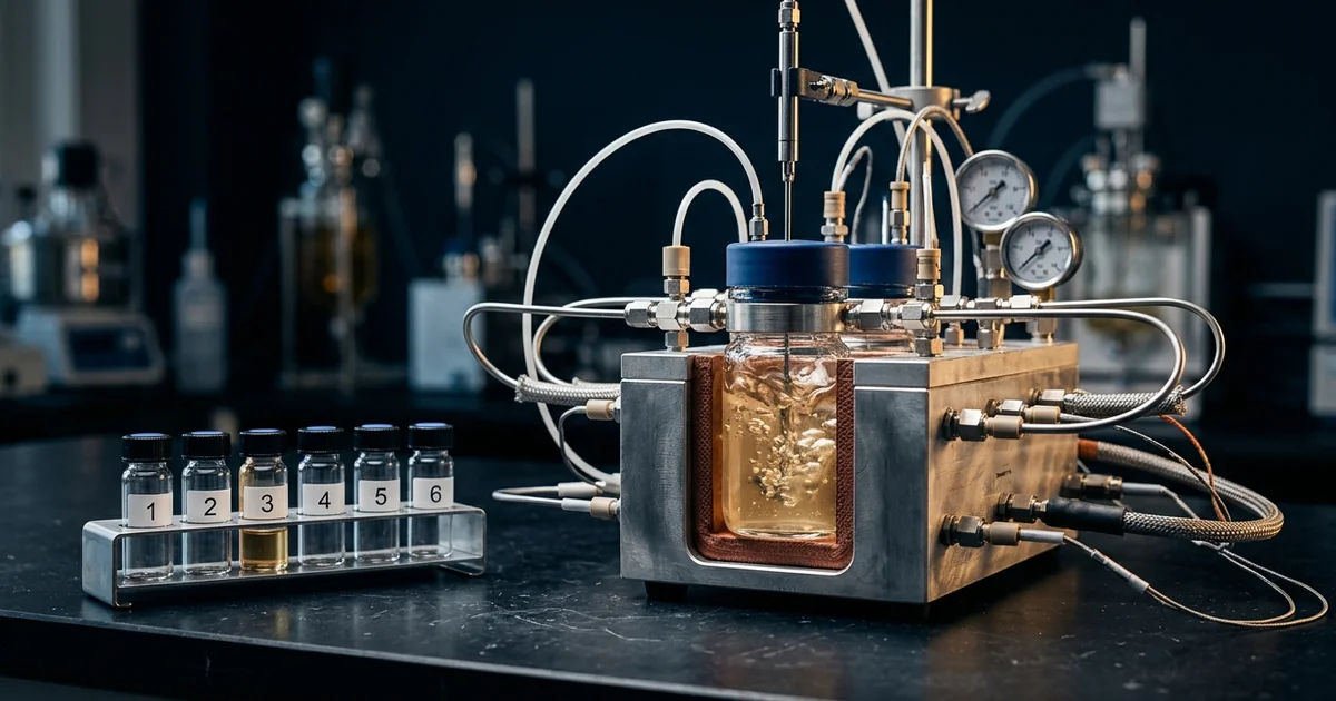
A reaction finishes in two hours at the bench, and the plant needs five or overshoots its temperature limit. The bench data were real, so the surprise comes from what those data were asked to say. Reaction kinetics for scale-up means a tested rate law, a rate constant with its temperature dependence, and a clear view of what limits the rate at plant scale. Get any one wrong and batch time, cooling demand and yield all miss the case. This guide shows how to determine reaction order, extract rate constants and activation energy, and judge whether bench rates will survive the move to a larger vessel. It builds on our guides to scale-down models and reactor selection, within our chemical reaction engineering practice.
The Three Parts of Reaction Kinetics for Scale-Up: Rate Law, Rate Constant and Temperature
A kinetic model for scale-up answers one question: how fast does the reaction go under the conditions the plant will impose? It has three parts, and each part maps to a plant decision. The rate law gives the dependence on concentration, the rate constant sets the speed at one temperature, and the Arrhenius equation extends that speed across temperature. Rate laws are determined by experiment only, and OpenStax Chemistry 2e states they are not reliably predicted by reaction stoichiometry.
For a reaction of A with B, the rate law has the form rate = k[A]m[B]n. The exponents m and n are the reaction orders, and k is the rate constant. Its units depend on the overall order: s−1 for first order and mol−1 dm3 s−1 for second order, as the Wikipedia rate equation entry lists them.
| Kinetic quantity | What it sets at plant scale | Where it comes from |
|---|---|---|
| Reaction orders (m, n) | How batch time responds to charge concentration, dilution and dosing | Initial-rate, integrated-plot or half-life experiments |
| Rate constant (k) | Batch time at a given temperature, and the heat-release profile | Fit to concentration–time data at each temperature |
| Activation energy (Ea) | Sensitivity of the rate to temperature control and hot spots | Slope of the Arrhenius plot |
| Pre-exponential factor (A) | The absolute rate level at every temperature | Intercept of the Arrhenius plot |
| Rate-limiting step | Whether the bench rate is intrinsic or includes transport | Agitation, scale-down and Damköhler checks |
Heat follows rate. For an exothermic reaction, the heat release rate equals the reaction rate times the heat evolved per unit of reaction (−ΔHr) times the reaction volume. A wrong rate law therefore means a wrong cooling duty. Our guide to reaction calorimetry and scale-up thermal data shows how the two are measured together. The next section starts with reaction order, because everything that depends on concentration depends on it.
Reaction Order and Rate Law Determination: Initial Rates, Integrated Plots and Half-Life
Reaction order determination decides how batch time responds to every change in charge concentration, solvent ratio or dosing profile. A wrong order carries into every plant decision that depends on concentration. Four laboratory methods measure it, and they cross-check one another. Using at least two before a scale-up decision is cheap insurance.
| Method | What you measure | What the result shows | Watch-out |
|---|---|---|---|
| Initial rate method | The rate in the first minutes of several runs with different starting concentrations | The order in each reactant, from how the rate responds to its starting concentration (OpenStax) | Needs accurate early-time data and no induction period |
| Integrated rate plots | Concentration against time over a full run | A straight line of ln[A] against t means first order; 1/[A] against t means second order; [A] against t means zero order (OpenStax) | A narrow conversion range cannot separate the orders |
| Half-life method | The time to halve a concentration, at several starting concentrations | First-order half-life is independent of concentration (0.693/k); second order gives 1/(k[A]0); zero order gives [A]0/(2k) | Needs runs at two or more starting concentrations |
| Pseudo-first-order kinetics (flooding) | One reactant held in large excess so its concentration stays constant | The order in the other reactant, with k′ = k[B] (Wikipedia) | The excess changes the medium, so check the order in B separately |
How Reaction Order Changes Batch Time at Scale
Order decides whether a more concentrated charge shortens the batch. For a first-order reaction, the time to reach a given conversion does not depend on the starting concentration. For zero-order and second-order reactions it does, in opposite directions. The table uses the integrated rate laws to show the time to 90% conversion.
| Order | Time to 90% conversion | Effect of doubling the starting concentration [A]0 |
|---|---|---|
| Zero | 0.9[A]0/k | Time doubles |
| First | ln 10/k = 2.303/k | Time unchanged |
| Second | 9/(k[A]0) | Time halves |
Derived from the integrated rate laws in OpenStax Chemistry 2e; 90% conversion means [A] = 0.1[A]0.
Take a second-order reaction with an assumed k = 0.02 L mol−1 min−1. At 1.0 mol/L it needs 9 ÷ (0.02 × 1.0) = 450 min to reach 90%, and at 2.0 mol/L it needs 225 min. A first-order reaction with a 30 min half-life needs about 100 min at either concentration (2.303 ÷ 0.0231 min−1). These numbers are assumptions chosen to show the method.
The plant consequence is direct. A throughput-raising move to a more concentrated charge speeds up a second-order step, leaves a first-order step unchanged and slows a zero-order step. At equal half-lives, first order reaches 99% conversion in 6.6 half-lives, whereas second order needs 99, so tight conversion specifications on a second-order step dominate cycle time. Order tells you how the rate responds to concentration, and temperature is the other lever.
The Arrhenius Equation for Process Scale-Up: Activation Energy and Temperature Sensitivity
The Arrhenius equation describes the rate constant temperature dependence, and it explains why small temperature differences produce large differences in conversion. Svante Arrhenius proposed the relationship in his 1889 paper on the inversion of cane sugar by acids. In modern form, k = A e−Ea/RT, where A is the pre-exponential factor, Ea is the activation energy, R is the molar gas constant and T is the absolute temperature. OpenStax defines activation energy as the minimum energy necessary to form a product during a collision between reactants.
Plotting ln k against 1/T gives a straight line of slope −Ea/R, and the two-point form is ln(k2/k1) = (Ea/R)(1/T1 − 1/T2). NIST lists the molar gas constant as exactly 8.314 462 618… J mol−1 K−1. Keep Ea in J/mol when R is in J mol−1 K−1, or the exponent is wrong by a factor of 1,000.
| Activation energy (kJ/mol) | k(310 K) / k(300 K) | k(360 K) / k(350 K) |
|---|---|---|
| 30 | 1.47 | 1.33 |
| 50 | 1.91 | 1.61 |
| 80 | 2.81 | 2.15 |
| 120 | 4.72 | 3.14 |
Illustrative arithmetic from the Arrhenius equation with R = 8.314 J mol−1 K−1. The activation energies are chosen to show the range, not measured values.
The familiar rule that the rate doubles every 10 K is a special case. Near 300 K it needs an activation energy of about 54 kJ/mol, and near 350 K it needs about 73 kJ/mol. Reactions with higher activation energy are more temperature-sensitive than the rule implies, and those with lower activation energy are less.
Temperature control tolerance therefore becomes a quality parameter. Take an activation energy of 80 kJ/mol at 350 K. Running 5 K above the set point raises the rate constant by a factor of 1.47, and running 5 K below cuts it to 0.67. That 10 K band spans a 2.2-fold rate range, and a poorly mixed vessel with hot and cold zones inside the band produces batch-to-batch differences in conversion.
Activation energy from lab data is only as good as the temperature range behind it. A two-point fit always produces a line, so use at least three temperatures to test whether the Arrhenius plot is straight. Extrapolation magnifies error. Consider a fit anchored at 343 K and extended 20 K to 363 K. An activation energy of 60 kJ/mol predicts a 3.2-fold rate increase, and an error of ±10 kJ/mol moves that prediction between 2.6 and 3.9. The next section explains why even a well-measured rate constant can fail to predict the plant.
Intrinsic vs Apparent Kinetics: Why Kinetics Change on Scale-Up
In reaction kinetics for scale-up, the rate constant belongs to the chemistry, and the observed rate belongs to the chemistry plus the vessel. Intrinsic kinetics describe the reaction with no transport effects, while apparent kinetics describe what a given reactor delivers once mixing, heat transfer or mass transfer take part. Scaling up changes the vessel and leaves the chemistry unchanged. Any change in observed rate is therefore a transport effect or a feed effect.
| Attribute | Intrinsic kinetics | Apparent kinetics |
|---|---|---|
| What it describes | The chemical step alone | The chemical step plus mixing, heat and mass transfer |
| Responds to agitation | No | Yes, when transport limits the rate |
| Temperature sensitivity | Set by the activation energy of the reaction | Lower when a transport step limits, since diffusion varies far less with temperature |
| Changes with scale | No | Yes, because the vessel changes |
| Use in scale-up | The number that carries across to the plant | A measurement of one vessel, not a design basis |
The Damköhler number (Da) compares the two. Wikipedia’s entry defines the first Damköhler number as the reaction rate divided by the convective mass transport rate. For a reaction of order n it equals kC0n−1τ, with inlet concentration C0 and residence time τ. When Da is large, the reaction is much faster than the transport, so transport sets the observed rate. Bosman’s list of problems that appear at scale in The Chemical Engineer opens with non-linear mixing effects and heat-transfer limitations, both transport effects.
Four checks separate chemistry from transport at bench scale:
- Change the agitation — an intrinsic rate does not respond to stirrer speed, so a rate that does has transport in it.
- Read the activation energy — a low apparent value points to transport control. A step with an effective activation energy of 15 kJ/mol gains only a factor of 1.15 for 10 K at 350 K.
- Reproduce plant mixing — run a scale-down model that matches the plant’s mixing time and heat-removal ratio.
- Test catalysed systems formally — the Weisz–Prater and Madon–Boudart criteria check whether measured rates of heterogeneous catalytic reactions are free of transport artifacts.
Heat transfer adds its own scale effect. For vessels of the same shape, the jacket area per unit volume falls as the inverse of the linear dimension. A tenfold volume increase leaves 46% of the bench value, as our guide to pilot plant sizing works out. A rate constant measured free of transport carries over, and one that already contains transport does not. Our comparison of homogeneous and heterogeneous catalysis covers where the catalyst phase adds its own transport step.
Isothermal vs Non-Isothermal Kinetic Study: Choosing the Experiment
The experiment you choose determines which kinetic quantities you can trust in reaction kinetics for scale-up. Isothermal studies hold the temperature constant and give one clean rate constant per run. Non-isothermal studies sweep temperature and extract kinetic parameters from fewer experiments, at the price of assumptions about the model. Reaction calorimetry sits between them by following heat flow in a stirred, controlled vessel.
| Approach | How the rate is observed | Strength | Limitation |
|---|---|---|---|
| Isothermal batch series | Concentration against time at three or more fixed temperatures | Direct k at each temperature, a straightness check on the Arrhenius plot, and order from the methods above | A fast exotherm makes a truly isothermal run hard, and sampling lags the reaction |
| Non-isothermal differential scanning calorimetry (DSC) at several heating rates | Heat flow against temperature | Fast activation-energy screening; ASTM E698 applies the Flynn/Wall/Ozawa method to DSC curves at different heating rates | Assumes the reaction follows the Arrhenius equation and a general rate law |
| Reaction calorimetry | Heat flow in a stirred, jacketed vessel under plant-like dosing | A rate profile under realistic mixing, with the heat of reaction in the same experiment | Reads heat as rate, so it needs the heat of reaction and a closed heat balance |
The ICTAC Kinetics Committee has published recommendations for performing kinetic computations and for collecting the experimental data in thermal analysis. Both are worth reading before committing to a non-isothermal programme. Use the isothermal series as the reference and the thermal or calorimetric data as the cross-check. When all three agree on activation energy, the model is ready for a larger vessel. When they disagree, find out why before scaling, because a second reaction or a transport effect is the usual cause.
Troubleshooting: Why the Reaction Is Slower or Less Consistent at Plant Scale
Kinetic surprises at the plant have a short list of causes, and most are visible in the bench data once you know where to look. The symptom tells you which part of the kinetic model failed. Each item below pairs a symptom with its usual cause and its consequence. Working through them in order avoids chasing the rate constant when the vessel is the problem.
- Reaction slower at plant scale than lab — transport now limits the rate, or the bulk runs cooler than the bench because heating lags in a larger vessel. Batch time lengthens and capacity falls.
- Unexpected reaction rate change — a raw-material lot carries inhibitors or catalytic impurities that analytical-grade bench reagents lacked, a case of the feedstock variability Bosman lists. The rate shifts in a way no temperature change explains.
- Inconsistent conversion between batches — the temperature band is wide for the activation energy, charge concentration drifts on a non-first-order reaction, or sample timing varies. Off-spec lots and rework follow.
- Kinetics do not scale — the rate law was copied from stoichiometry or fitted over a narrow range. The batch-time prediction fails on the first plant batch.
- Rate constant from lab does not fit plant data — transport effects were folded into the bench value, or the plant temperature profile differs from the isothermal bench runs. Refitting on plant data then costs production batches.
- Rate runs ahead of cooling — a high activation energy and a fast feed let the temperature rise faster than the jacket removes heat. The batch overshoots, which makes adiabatic temperature rise data part of the kinetic basis.
Read each symptom as a question about one kinetic quantity from the first table. That turns a vague scale-up failure into a short, ordered list of experiments, and the last section turns that list into a checklist.
Kinetics Scale-Up Checklist: Five Questions Before the First Plant Batch
Five questions turn a set of bench experiments into scale-up kinetics you can defend in a review. They follow the sections above, so each answer feeds the next. The output is a one-page kinetic summary that belongs in the technology transfer package. A question you cannot answer marks the experiment to run next.
- Is the rate law measured, not assumed? — At least two of the methods in the order table agree.
- Is k measured at three or more temperatures across the plant range? — The Arrhenius plot is straight, and the plant will not run far outside it.
- Is the bench rate intrinsic? — An agitation test, a Damköhler check or a scale-down run says so.
- Does the plant temperature band keep the rate inside tolerance? — Apply the Arrhenius ratio for your activation energy to the control band.
- Does heat release match cooling capacity? — Heat release is the rate times the heat of reaction, calorimetry measures it directly, and it sizes the cooling duty.
Reaction kinetics for scale-up is ready for the plant when all five questions have answers. If questions 1 to 3 are open, the next step is more bench work, not a pilot. Questions 4 and 5 close with arithmetic and calorimetry. A pilot plant sizing decision comes only when real feedstock, solids or long-run effects remain unknown after all five answers.
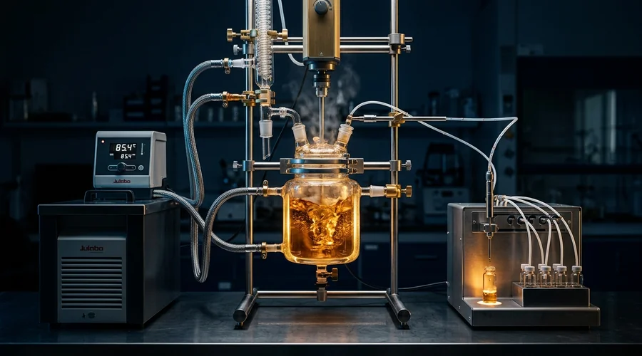
A reaction engineering consultant adds most value before the experiments are run, by choosing the few that settle the kinetic model. For producers in India and the Middle East moving a route from bench to plant, that planning decides the schedule. Our process development consulting team provides chemical process development services, including reaction kinetics for scale-up studies and contract process development. Our scale-up support works as a scale-up partner and delivers pilot plant support, and our lab-to-market service carries the chosen route through technology transfer, including R&D outsourcing for chemical manufacturing.
Frequently Asked Questions
What is the Arrhenius equation used for?
The Arrhenius equation, k = A exp(−Ea/RT), relates a rate constant to absolute temperature. In process work it serves two purposes. Plotting ln k against 1/T for rate constants measured at several temperatures gives the activation energy and pre-exponential factor. The fitted equation then predicts the rate constant at other temperatures within the tested range.
Its plant value is in temperature tolerance. For an activation energy of 80 kJ/mol at 350 K, a 10 K rise multiplies the rate constant by 2.15. Extrapolating well beyond the measured range magnifies any error in the activation energy, so measure across the range the plant will use.
How do you determine reaction order experimentally?
Measure rates and fit them, because stoichiometry does not give the order. The initial rate method compares rates from runs with different starting concentrations. Integrated plots test whether ln[A], 1/[A] or [A] falls linearly with time, which indicates first, second or zero order. The half-life method checks how the time to halve a concentration changes with the starting concentration.
Use at least two methods and compare. Where one reactant is in large excess, the pseudo-first-order method isolates the order in the other. Agreement between methods is the evidence that the rate law will carry to a larger vessel.
Why does my reaction slow down at plant scale?
The rate constant does not change with scale, so the cause is either transport or feed. A larger vessel mixes more slowly and removes heat less effectively per unit volume, which can make mixing or heat transfer limit the observed rate. The bulk temperature can also sit below the jacket set point because heating lags.
The other cause is raw material. Industrial lots carry impurities that analytical-grade bench reagents lack, and some inhibit the reaction. Test by changing agitation at the bench, running a scale-down model with plant mixing time, and repeating the bench run with the plant raw material.
What is the difference between intrinsic and apparent kinetics?
Intrinsic kinetics describe the chemical step alone, free of mixing, heat-transfer and mass-transfer effects. Apparent kinetics describe the rate a specific reactor delivers, which includes those effects. Only the intrinsic rate constant carries from bench to plant, because the vessel changes with scale and the chemistry does not.
Signs of apparent kinetics are a rate that responds to stirrer speed and an unusually low activation energy. For catalysed systems, the Weisz–Prater and Madon–Boudart criteria give formal tests for transport artifacts.
What is activation energy, and how many temperatures do you need to measure it?
Activation energy is the minimum energy needed for reactants to form products in a collision. In practice it is the negative of the Arrhenius plot slope multiplied by the gas constant. It tells you how steeply the rate rises with temperature. A high value means tight temperature control matters.
Use at least three temperatures. Two points always fit a straight line, so only a third point tests whether the Arrhenius relationship holds. Span as wide a range as the chemistry allows, and keep the plant operating window inside it.
First order vs second order reaction: what changes at scale?
A first-order reaction has a half-life that does not depend on concentration, so its time to a given conversion does not change with charge concentration. A second-order reaction has a half-life of 1/(k[A]0), so doubling the starting concentration halves the time to a given conversion.
The tail differs as well. At equal half-lives, the time to 90% conversion is 3.3 half-lives for first order and 9 for second order. A second-order step therefore punishes tight conversion specifications far more heavily, since 99% conversion takes 6.6 half-lives at first order and 99 at second order.
Should you use an isothermal or non-isothermal kinetic study?
Use both, with the isothermal series as the reference. Isothermal runs at three or more temperatures give direct rate constants and a check on the Arrhenius plot. Non-isothermal methods such as DSC at several heating rates, as in ASTM E698, screen activation energy quickly. They assume the reaction follows the Arrhenius equation and a general rate law.
Reaction calorimetry adds a rate profile under plant-like mixing and dosing. If the three disagree on activation energy, find out why before scaling, since a second reaction or a transport effect is the usual cause.
How tightly does plant temperature need to be controlled?
It depends on the activation energy and on how much conversion variation the specification tolerates. At 350 K with an activation energy of 80 kJ/mol, a band of ±5 K spans a rate range from 0.67 to 1.47 times the set-point value, a 2.2-fold spread. At 30 kJ/mol the same band gives a much narrower spread.
Convert your measured activation energy into a rate band, compare it with the conversion tolerance, and set the control band from that comparison. Poor mixing widens the real band because local temperatures differ from the probe reading.
Preparing Kinetic Data for a Scale-Up Decision?
Global Formulation provides route selection, process development and scale-up partnership, from designing the kinetic study and reading the Arrhenius data to pilot plant support, technology transfer and R&D outsourcing for chemical manufacturing.
Talk to Our Process Team